# 多分类任务

/**
 * @license
 * Copyright 2018 Google LLC. All Rights Reserved.
 * Licensed under the Apache License, Version 2.0 (the "License");
 * you may not use this file except in compliance with the License.
 * You may obtain a copy of the License at
 *
 * http://www.apache.org/licenses/LICENSE-2.0
 *
 * Unless required by applicable law or agreed to in writing, software
 * distributed under the License is distributed on an "AS IS" BASIS,
 * WITHOUT WARRANTIES OR CONDITIONS OF ANY KIND, either express or implied.
 * See the License for the specific language governing permissions and
 * limitations under the License.
 * =============================================================================
 */

import * as tf from "@tensorflow/tfjs";

export const IRIS_CLASSES = ["山鸢尾", "变色鸢尾", "维吉尼亚鸢尾"];
export const IRIS_NUM_CLASSES = IRIS_CLASSES.length;

// Iris flowers data. Source:
//   https://archive.ics.uci.edu/ml/machine-learning-databases/iris/iris.data
const IRIS_DATA = [
  [5.1, 3.5, 1.4, 0.2, 0],
  [4.9, 3.0, 1.4, 0.2, 0],
  [4.7, 3.2, 1.3, 0.2, 0],
  [4.6, 3.1, 1.5, 0.2, 0],
  [5.0, 3.6, 1.4, 0.2, 0],
  [5.4, 3.9, 1.7, 0.4, 0],
  [4.6, 3.4, 1.4, 0.3, 0],
  [5.0, 3.4, 1.5, 0.2, 0],
  [4.4, 2.9, 1.4, 0.2, 0],
  [4.9, 3.1, 1.5, 0.1, 0],
  [5.4, 3.7, 1.5, 0.2, 0],
  [4.8, 3.4, 1.6, 0.2, 0],
  [4.8, 3.0, 1.4, 0.1, 0],
  [4.3, 3.0, 1.1, 0.1, 0],
  [5.8, 4.0, 1.2, 0.2, 0],
  [5.7, 4.4, 1.5, 0.4, 0],
  [5.4, 3.9, 1.3, 0.4, 0],
  [5.1, 3.5, 1.4, 0.3, 0],
  [5.7, 3.8, 1.7, 0.3, 0],
  [5.1, 3.8, 1.5, 0.3, 0],
  [5.4, 3.4, 1.7, 0.2, 0],
  [5.1, 3.7, 1.5, 0.4, 0],
  [4.6, 3.6, 1.0, 0.2, 0],
  [5.1, 3.3, 1.7, 0.5, 0],
  [4.8, 3.4, 1.9, 0.2, 0],
  [5.0, 3.0, 1.6, 0.2, 0],
  [5.0, 3.4, 1.6, 0.4, 0],
  [5.2, 3.5, 1.5, 0.2, 0],
  [5.2, 3.4, 1.4, 0.2, 0],
  [4.7, 3.2, 1.6, 0.2, 0],
  [4.8, 3.1, 1.6, 0.2, 0],
  [5.4, 3.4, 1.5, 0.4, 0],
  [5.2, 4.1, 1.5, 0.1, 0],
  [5.5, 4.2, 1.4, 0.2, 0],
  [4.9, 3.1, 1.5, 0.1, 0],
  [5.0, 3.2, 1.2, 0.2, 0],
  [5.5, 3.5, 1.3, 0.2, 0],
  [4.9, 3.1, 1.5, 0.1, 0],
  [4.4, 3.0, 1.3, 0.2, 0],
  [5.1, 3.4, 1.5, 0.2, 0],
  [5.0, 3.5, 1.3, 0.3, 0],
  [4.5, 2.3, 1.3, 0.3, 0],
  [4.4, 3.2, 1.3, 0.2, 0],
  [5.0, 3.5, 1.6, 0.6, 0],
  [5.1, 3.8, 1.9, 0.4, 0],
  [4.8, 3.0, 1.4, 0.3, 0],
  [5.1, 3.8, 1.6, 0.2, 0],
  [4.6, 3.2, 1.4, 0.2, 0],
  [5.3, 3.7, 1.5, 0.2, 0],
  [5.0, 3.3, 1.4, 0.2, 0],
  [7.0, 3.2, 4.7, 1.4, 1],
  [6.4, 3.2, 4.5, 1.5, 1],
  [6.9, 3.1, 4.9, 1.5, 1],
  [5.5, 2.3, 4.0, 1.3, 1],
  [6.5, 2.8, 4.6, 1.5, 1],
  [5.7, 2.8, 4.5, 1.3, 1],
  [6.3, 3.3, 4.7, 1.6, 1],
  [4.9, 2.4, 3.3, 1.0, 1],
  [6.6, 2.9, 4.6, 1.3, 1],
  [5.2, 2.7, 3.9, 1.4, 1],
  [5.0, 2.0, 3.5, 1.0, 1],
  [5.9, 3.0, 4.2, 1.5, 1],
  [6.0, 2.2, 4.0, 1.0, 1],
  [6.1, 2.9, 4.7, 1.4, 1],
  [5.6, 2.9, 3.6, 1.3, 1],
  [6.7, 3.1, 4.4, 1.4, 1],
  [5.6, 3.0, 4.5, 1.5, 1],
  [5.8, 2.7, 4.1, 1.0, 1],
  [6.2, 2.2, 4.5, 1.5, 1],
  [5.6, 2.5, 3.9, 1.1, 1],
  [5.9, 3.2, 4.8, 1.8, 1],
  [6.1, 2.8, 4.0, 1.3, 1],
  [6.3, 2.5, 4.9, 1.5, 1],
  [6.1, 2.8, 4.7, 1.2, 1],
  [6.4, 2.9, 4.3, 1.3, 1],
  [6.6, 3.0, 4.4, 1.4, 1],
  [6.8, 2.8, 4.8, 1.4, 1],
  [6.7, 3.0, 5.0, 1.7, 1],
  [6.0, 2.9, 4.5, 1.5, 1],
  [5.7, 2.6, 3.5, 1.0, 1],
  [5.5, 2.4, 3.8, 1.1, 1],
  [5.5, 2.4, 3.7, 1.0, 1],
  [5.8, 2.7, 3.9, 1.2, 1],
  [6.0, 2.7, 5.1, 1.6, 1],
  [5.4, 3.0, 4.5, 1.5, 1],
  [6.0, 3.4, 4.5, 1.6, 1],
  [6.7, 3.1, 4.7, 1.5, 1],
  [6.3, 2.3, 4.4, 1.3, 1],
  [5.6, 3.0, 4.1, 1.3, 1],
  [5.5, 2.5, 4.0, 1.3, 1],
  [5.5, 2.6, 4.4, 1.2, 1],
  [6.1, 3.0, 4.6, 1.4, 1],
  [5.8, 2.6, 4.0, 1.2, 1],
  [5.0, 2.3, 3.3, 1.0, 1],
  [5.6, 2.7, 4.2, 1.3, 1],
  [5.7, 3.0, 4.2, 1.2, 1],
  [5.7, 2.9, 4.2, 1.3, 1],
  [6.2, 2.9, 4.3, 1.3, 1],
  [5.1, 2.5, 3.0, 1.1, 1],
  [5.7, 2.8, 4.1, 1.3, 1],
  [6.3, 3.3, 6.0, 2.5, 2],
  [5.8, 2.7, 5.1, 1.9, 2],
  [7.1, 3.0, 5.9, 2.1, 2],
  [6.3, 2.9, 5.6, 1.8, 2],
  [6.5, 3.0, 5.8, 2.2, 2],
  [7.6, 3.0, 6.6, 2.1, 2],
  [4.9, 2.5, 4.5, 1.7, 2],
  [7.3, 2.9, 6.3, 1.8, 2],
  [6.7, 2.5, 5.8, 1.8, 2],
  [7.2, 3.6, 6.1, 2.5, 2],
  [6.5, 3.2, 5.1, 2.0, 2],
  [6.4, 2.7, 5.3, 1.9, 2],
  [6.8, 3.0, 5.5, 2.1, 2],
  [5.7, 2.5, 5.0, 2.0, 2],
  [5.8, 2.8, 5.1, 2.4, 2],
  [6.4, 3.2, 5.3, 2.3, 2],
  [6.5, 3.0, 5.5, 1.8, 2],
  [7.7, 3.8, 6.7, 2.2, 2],
  [7.7, 2.6, 6.9, 2.3, 2],
  [6.0, 2.2, 5.0, 1.5, 2],
  [6.9, 3.2, 5.7, 2.3, 2],
  [5.6, 2.8, 4.9, 2.0, 2],
  [7.7, 2.8, 6.7, 2.0, 2],
  [6.3, 2.7, 4.9, 1.8, 2],
  [6.7, 3.3, 5.7, 2.1, 2],
  [7.2, 3.2, 6.0, 1.8, 2],
  [6.2, 2.8, 4.8, 1.8, 2],
  [6.1, 3.0, 4.9, 1.8, 2],
  [6.4, 2.8, 5.6, 2.1, 2],
  [7.2, 3.0, 5.8, 1.6, 2],
  [7.4, 2.8, 6.1, 1.9, 2],
  [7.9, 3.8, 6.4, 2.0, 2],
  [6.4, 2.8, 5.6, 2.2, 2],
  [6.3, 2.8, 5.1, 1.5, 2],
  [6.1, 2.6, 5.6, 1.4, 2],
  [7.7, 3.0, 6.1, 2.3, 2],
  [6.3, 3.4, 5.6, 2.4, 2],
  [6.4, 3.1, 5.5, 1.8, 2],
  [6.0, 3.0, 4.8, 1.8, 2],
  [6.9, 3.1, 5.4, 2.1, 2],
  [6.7, 3.1, 5.6, 2.4, 2],
  [6.9, 3.1, 5.1, 2.3, 2],
  [5.8, 2.7, 5.1, 1.9, 2],
  [6.8, 3.2, 5.9, 2.3, 2],
  [6.7, 3.3, 5.7, 2.5, 2],
  [6.7, 3.0, 5.2, 2.3, 2],
  [6.3, 2.5, 5.0, 1.9, 2],
  [6.5, 3.0, 5.2, 2.0, 2],
  [6.2, 3.4, 5.4, 2.3, 2],
  [5.9, 3.0, 5.1, 1.8, 2]
];

/**
 * Convert Iris data arrays to `tf.Tensor`s.
 *
 * @param data The Iris input feature data, an `Array` of `Array`s, each element
 *   of which is assumed to be a length-4 `Array` (for petal length, petal
 *   width, sepal length, sepal width).
 * @param targets An `Array` of numbers, with values from the set {0, 1, 2}:
 *   representing the true category of the Iris flower. Assumed to have the same
 *   array length as `data`.
 * @param testSplit Fraction of the data at the end to split as test data: a
 *   number between 0 and 1.
 * @return A length-4 `Array`, with
 *   - training data as `tf.Tensor` of shape [numTrainExapmles, 4].
 *   - training one-hot labels as a `tf.Tensor` of shape [numTrainExamples, 3]
 *   - test data as `tf.Tensor` of shape [numTestExamples, 4].
 *   - test one-hot labels as a `tf.Tensor` of shape [numTestExamples, 3]
 */
function convertToTensors(data, targets, testSplit) {
  const numExamples = data.length;
  if (numExamples !== targets.length) {
    throw new Error("data and split have different numbers of examples");
  }

  // Randomly shuffle `data` and `targets`.
  const indices = [];
  for (let i = 0; i < numExamples; ++i) {
    indices.push(i);
  }
  tf.util.shuffle(indices);

  const shuffledData = [];
  const shuffledTargets = [];
  for (let i = 0; i < numExamples; ++i) {
    shuffledData.push(data[indices[i]]);
    shuffledTargets.push(targets[indices[i]]);
  }

  // Split the data into a training set and a tet set, based on `testSplit`.
  const numTestExamples = Math.round(numExamples * testSplit);
  const numTrainExamples = numExamples - numTestExamples;

  const xDims = shuffledData[0].length;

  // Create a 2D `tf.Tensor` to hold the feature data.
  const xs = tf.tensor2d(shuffledData, [numExamples, xDims]);

  // Create a 1D `tf.Tensor` to hold the labels, and convert the number label
  // from the set {0, 1, 2} into one-hot encoding (.e.g., 0 --> [1, 0, 0]).
  const ys = tf.oneHot(tf.tensor1d(shuffledTargets).toInt(), IRIS_NUM_CLASSES);

  // Split the data into training and test sets, using `slice`.
  const xTrain = xs.slice([0, 0], [numTrainExamples, xDims]);
  const xTest = xs.slice([numTrainExamples, 0], [numTestExamples, xDims]);
  const yTrain = ys.slice([0, 0], [numTrainExamples, IRIS_NUM_CLASSES]);
  const yTest = ys.slice([0, 0], [numTestExamples, IRIS_NUM_CLASSES]);
  return [xTrain, yTrain, xTest, yTest];
}

/**
 * Obtains Iris data, split into training and test sets.
 *
 * @param testSplit Fraction of the data at the end to split as test data: a
 *   number between 0 and 1.
 *
 * @param return A length-4 `Array`, with
 *   - training data as an `Array` of length-4 `Array` of numbers.
 *   - training labels as an `Array` of numbers, with the same length as the
 *     return training data above. Each element of the `Array` is from the set
 *     {0, 1, 2}.
 *   - test data as an `Array` of length-4 `Array` of numbers.
 *   - test labels as an `Array` of numbers, with the same length as the
 *     return test data above. Each element of the `Array` is from the set
 *     {0, 1, 2}.
 */
export function getIrisData(testSplit) {
  return tf.tidy(() => {
    const dataByClass = [];
    const targetsByClass = [];
    for (let i = 0; i < IRIS_CLASSES.length; ++i) {
      dataByClass.push([]);
      targetsByClass.push([]);
    }
    for (const example of IRIS_DATA) {
      const target = example[example.length - 1];
      const data = example.slice(0, example.length - 1);
      dataByClass[target].push(data);
      targetsByClass[target].push(target);
    }

    const xTrains = [];
    const yTrains = [];
    const xTests = [];
    const yTests = [];
    for (let i = 0; i < IRIS_CLASSES.length; ++i) {
      const [xTrain, yTrain, xTest, yTest] = convertToTensors(
        dataByClass[i],
        targetsByClass[i],
        testSplit
      );
      xTrains.push(xTrain);
      yTrains.push(yTrain);
      xTests.push(xTest);
      yTests.push(yTest);
    }

    const concatAxis = 0;
    return [
      tf.concat(xTrains, concatAxis),
      tf.concat(yTrains, concatAxis),
      tf.concat(xTests, concatAxis),
      tf.concat(yTests, concatAxis)
    ];
  });
}

import { getIrisData, IRIS_CLASSES } from "./data";

window.onload = () => {
  // 按顺序获取 训练集数据 Train  验证集Test     getIrisDate()的参数是验证集的比例 有15%用于验证集
  const [xTrain, yTrain, xTest, yTest] = getIrisData(0.15);
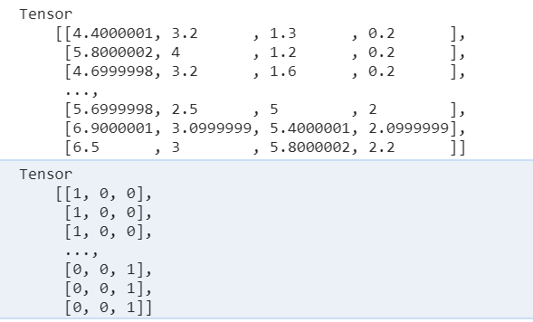
  xTrain.print();
  yTrain.print();
};

import * as tf from "@tensorflow/tfjs";
import { getIrisData, IRIS_CLASSES } from "./data";
import { mod } from "@tensorflow/tfjs";

window.onload = () => {
  // 按顺序获取 训练集数据 Train  验证集Test     getIrisDate()的参数是验证集的比例 有15%用于验证集
  const [xTrain, yTrain, xTest, yTest] = getIrisData(0.15);
  const model = tf.sequential();
  // 添加中间层，凭感觉设置十个神经元
  model.add(
    tf.layers.dense({
      units: 10,
      inputShape: [xTrain.shape[1]],
      activation: "sigmoid"
    })
  );
  // 多分类神经网络的核心，输出是三个神经元，使用softmax激活函数可以分别算出每个类别的概率
  model.add(
    tf.layers.dense({
      units: 3,
      activation: "softmax"
    })
  );
};

import * as tf from "@tensorflow/tfjs";
import * as tfvis from "@tensorflow/tfjs-vis";
import { getIrisData, IRIS_CLASSES } from "./data";

window.onload = async () => {
  // 按顺序获取 训练集数据 Train  验证集Test     getIrisDate()的参数是验证集的比例 有15%用于验证集
  const [xTrain, yTrain, xTest, yTest] = getIrisData(0.15);
  const model = tf.sequential();
  // 添加中间层，凭感觉设置十个神经元
  model.add(
    tf.layers.dense({
      units: 10,
      inputShape: [xTrain.shape[1]],
      activation: "sigmoid"
    })
  );
  // 多分类神经网络的核心，输出是三个神经元，使用softmax激活函数可以分别算出每个类别的概率
  model.add(
    tf.layers.dense({
      units: 3,
      activation: "softmax"
    })
  );

  // 设置损失函数、优化器、及准确度
  model.compile({
    // 交叉熵
    loss: "categoricalCrossentropy",
    optimizer: tf.train.adam(0.1),
    // 准确度
    metrics: ["accuracy"]
  });

  // 训练模型
  await model.fit(xTrain, yTrain, {
    epochs: 100,
    // 添加验证集
    validationData: [xTest, yTest],
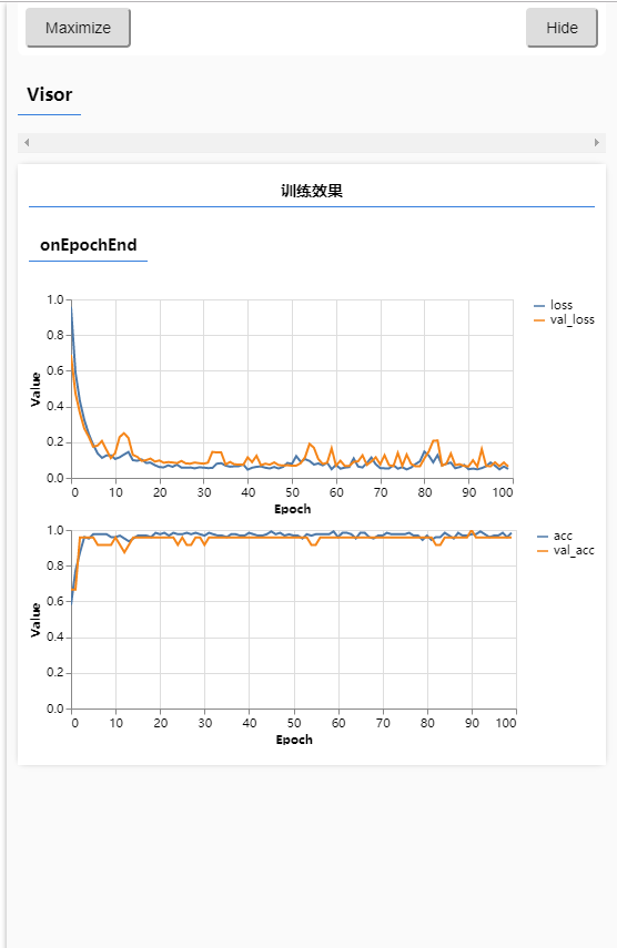
    callbacks: tfvis.show.fitCallbacks(
      { name: "训练效果" },
      // 显示训练过程的损失，验证集误差，准确度，验证集准确度
      ["loss", "val_loss", "acc", "val_acc"],
      { callbacks: ["onEpochEnd"] }
    )
  });
};

import * as tf from "@tensorflow/tfjs";
import * as tfvis from "@tensorflow/tfjs-vis";
import { getIrisData, IRIS_CLASSES } from "./data";

window.onload = async () => {
  // 按顺序获取 训练集数据 Train  验证集Test     getIrisDate()的参数是验证集的比例 有15%用于验证集
  const [xTrain, yTrain, xTest, yTest] = getIrisData(0.15);
  const model = tf.sequential();
  // 添加中间层，凭感觉设置十个神经元
  model.add(
    tf.layers.dense({
      units: 10,
      inputShape: [xTrain.shape[1]],
      activation: "sigmoid"
    })
  );
  // 多分类神经网络的核心，输出是三个神经元，使用softmax激活函数可以分别算出每个类别的概率
  model.add(
    tf.layers.dense({
      units: 3,
      activation: "softmax"
    })
  );

  // 设置损失函数、优化器、及准确度
  model.compile({
    // 交叉熵
    loss: "categoricalCrossentropy",
    optimizer: tf.train.adam(0.1),
    // 准确度
    metrics: ["accuracy"]
  });

  await model.fit(xTrain, yTrain, {
    epochs: 100,
    // 添加验证集
    validationData: [xTest, yTest],
    callbacks: tfvis.show.fitCallbacks(
      { name: "训练效果" },
      // 显示训练过程的损失，验证集误差，准确度，验证集准确度
      ["loss", "val_loss", "acc", "val_acc"],
      { callbacks: ["onEpochEnd"] }
    )
  });

  window.predict = form => {
    const input = tf.tensor([
      [form.a.value * 1, form.b.value * 1, form.c.value * 1, form.d.value * 1]
    ]);
    const pred = model.predict(input);
    // 在上面我们看到y的值是一个二维数组 [[0, 0, 1], [1, 0, 0]] 这样的数据结构
    // pred.argMax(1) 输出第1维也就是 [0,0,1] 的最大值 1 的坐标，正好对应着 IRIS_CLASSES数组的坐标
    alert(`预测结果：${IRIS_CLASSES[pred.argMax(1).dataSync(0)]}`);
  };
};